Repeated planning
1. Introduction to repeated planning
The problem facts used to create a solution may change before or during the execution of that solution. Delaying planning in order to lower the risk of problem facts changing is not ideal, as an incomplete plan is preferable to no plan.
The following examples demonstrate situations where planning solutions need to be altered due to unpredictable changes:
-
Unforeseen fact changes
-
An employee assigned to a shift calls in sick.
-
An airplane scheduled to take off has a technical delay.
-
One of the machines or vehicles break down.
Unforeseen fact changes benefit from using backup planning.
-
-
Cannot assign all entities immediately
Leave some unassigned. For example:
-
There are 10 shifts at the same time to assign but only nine employees to handle shifts.
For this type of planning, use overconstrained planning.
-
-
Unknown long term future facts
For example:
-
Hospital admissions for the next two weeks are reliable, but those for week three and four are less reliable, and for week five and beyond are not worth planning yet.
This problem benefits from continuous planning.
-
-
Constantly changing problem facts
Use real-time planning.
More CPU time results in a better planning solution.
OptaPy allows you to start planning earlier, despite unforeseen changes, as the optimization algorithms support planning a solution that has already been partially planned. This is known as repeated planning.
2. Backup planning
Backup planning adds extra score constraints to create space in the planning for when things go wrong. That creates a backup plan within the plan itself.
An example of backup planning is as follows:
-
Create an extra score constraint. For example:
-
Assign an employee as the spare employee (one for every 10 shifts at the same time).
-
Keep one hospital bed open in each department.
-
-
Change the planning problem when an unforeseen event occurs.
For example, if an employee calls in sick:
-
Delete the sick employee and leave their shifts unassigned.
-
Restart the planning, starting from that solution, which now has a different score.
-
The construction heuristics fills in the newly created gaps (probably with the spare employee) and the metaheuristics will improve it even further.
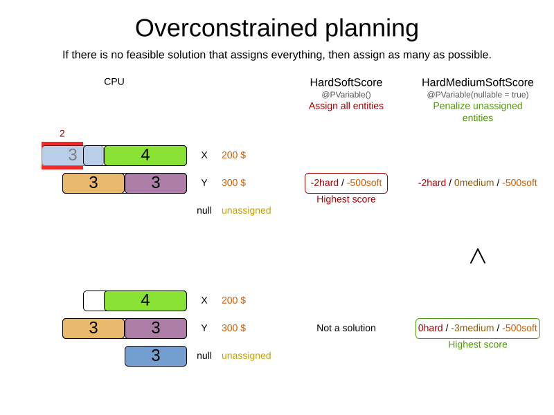
3. Overconstrained planning
When there is no feasible solution to assign all planning entities, it is preferable to assign as many entities as possible without breaking hard constraints. This is called overconstrained planning.
By default, OptaPy assigns all planning entities, overloads the planning values, and therefore breaks hard constraints. There are two ways to avoid this:
-
Use nullable planning variables, so that some entities are unassigned.
-
Add virtual values to catch the unassigned entities.
3.1. Overconstrained planning with nullable variables
If we handle overconstrained planning with nullable variables, the overload entities will be left unassigned:
To implement this:
-
Add a score level (usually a medium level between the hard and soft level) by switching
Scoretype. -
Make the planning variable nullable.
-
Add a score constraint on the new level (usually a medium constraint) to penalize the number of unassigned entities (or a weighted sum of them).
3.2. Overconstrained planning with virtual values
In overconstrained planning it is often useful to know which resources are lacking. In overconstrained planning with virtual values, the solution indicates which resources to buy.
To implement this:
-
Add an additional score level (usually a medium level between the hard and soft level) by switching
Scoretype. -
Add a number of virtual values. It can be difficult to determine a good formula to calculate that number:
-
Do not add too many, as that will decrease solver efficiency.
-
Importantly, do not add too few as that will lead to an infeasible solution.
-
-
Add a score constraint on the new level (usually a medium constraint) to penalize the number of virtual assigned entities (or a weighted sum of them).
-
Optionally, change all soft constraints to ignore virtual assigned entities.
4. Continuous planning (windowed planning)
Continuous planning is the technique of planning one or more upcoming planning periods at the same time and repeating that process monthly, weekly, daily, hourly, or even more frequently. However, as time is infinite, planning all future time periods is impossible.
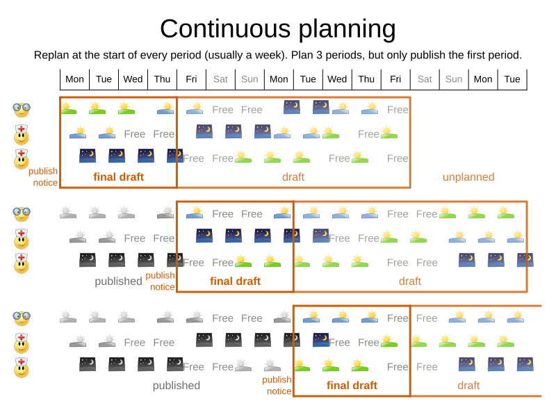
In the employee rostering example above, we re-plan every four days. Each time, we actually plan a window of 12 days, but we only publish the first four days, which is stable enough to share with the employees, so they can plan their social life accordingly.
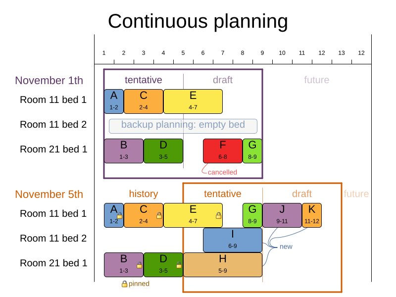
In the hospital bed planning example above, notice the difference between the original planning of November 1st and the new planning of November 5th: some problem facts (F, H, I, J, K) changed in the meantime, which results in unrelated planning entities (G) changing too.
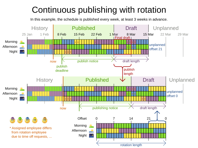
The planning window can be split up in several stages:
-
History
Immutable past time periods. It contains only pinned entities.
-
Recent historic entities can also affect score constraints that apply to movable entities. For example, in nurse rostering, a nurse that has worked the last three historic weekends in a row should not be assigned to three more weekends in a row, because she requires a one free weekend per month.
-
Do not load all historic entities in memory: even though pinned entities do not affect solving performance, they can cause out of memory problems when the data grows to years. Only load those that might still affect the current constraints with a good safety margin.
-
-
Published
Upcoming time periods that have been published. They contain only pinned and/or semi-movable planning entities.
-
The published schedule has been shared with the business. For example, in nurse rostering, the nurses will use this schedule to plan their personal lives, so they require a publish notice of for example 3 weeks in advance. Normal planning will not change that part of schedule.
Changing that schedule later is disruptive, but were exceptions force us to do them anyway (for example someone calls in sick), do change this part of the planning while minimizing disruption with non-disruptive replanning.
-
-
Draft
Upcoming time periods after the published time periods that can change freely. They contain movable planning entities, except for any that are pinned for other reasons (such as being pinned by a user).
-
The first part of the draft, called the final draft, will be published, so these planning entities can change one last time. The publishing frequency, for example once per week, determines the number of time periods that change from draft to published.
-
The latter time periods of the draft are likely change again in later planning efforts, especially if some of the problem facts change by then (for example nurse Ann doesn’t want to work on one of those days).
Despite that these latter planning entities might still change a lot, we can’t leave them out for later, because we would risk painting ourselves into a corner. For example, in employee rostering we could have all our rare skilled employees working the last 5 days of the week that gets published, which won’t reduce the score of that week, but will make it impossible for us to deliver a feasible schedule the next week. So the draft length needs to be longer than the part that will be published first.
-
That draft part is usually not shared with the business yet, because it is too volatile and it would only raise false expectations. However, it is stored in the database and used as a starting point for the next solver.
-
-
Unplanned (out of scope)
Planning entities that are not in the current planning window.
-
If the planning window is too small to plan all entities, you’re dealing with overconstrained planning.
-
If time is a planning variable, the size of the planning window is determined dynamically, in which case the unplanned stage is not applicable.
-
4.1. Pinned planning entities
A pinned planning entity doesn’t change during solving. This is commonly used by users to pin down one or more specific assignments and force OptaPlanner to schedule around those fixed assignments.
4.1.1. Pin down planning entities with @planning_pin
To pin some planning entities down, add an @planning_pin annotation on a bool getter of the planning entity class.
That boolean is True if the entity is pinned down to its current planning values and False otherwise.
-
Add the
@planning_pinannotation on abool:from optapy import planning_entity, planning_pin @planning_entity class Lecture: pinned: bool # ... @planning_pin def is_pinned(self): return self.pinned ...
In the example above, if pinned is True, the lecture will not be assigned to another period or room (even if the current period and rooms fields are None).
4.1.2. Configure a PinningFilter
Alternatively, to pin some planning entities down, create a predicate function that returns True if an entity is pinned, and False if it is movable.
This is more flexible and more verbose than the @planning_pin approach.
For example on the nurse rostering example:
-
Create the predicate function:
def shift_pinning_filter(solution, shift): return not solution.schedule_state.is_draft(shift) -
Configure the
pinning_filterof the@planning_entity:from optapy import planning_entity @planning_entity(pinning_filter=shift_pinning_filter) class Lecture: ...
4.2. Nonvolatile replanning to minimize disruption (semi-movable planning entities)
Replanning an existing plan can be very disruptive. If the plan affects humans (such as employees, drivers, …), very disruptive changes are often undesirable. In such cases, nonvolatile replanning helps by restricting planning freedom: the gain of changing a plan must be higher than the disruption it causes. This is usually implemented by taxing all planning entities that change.
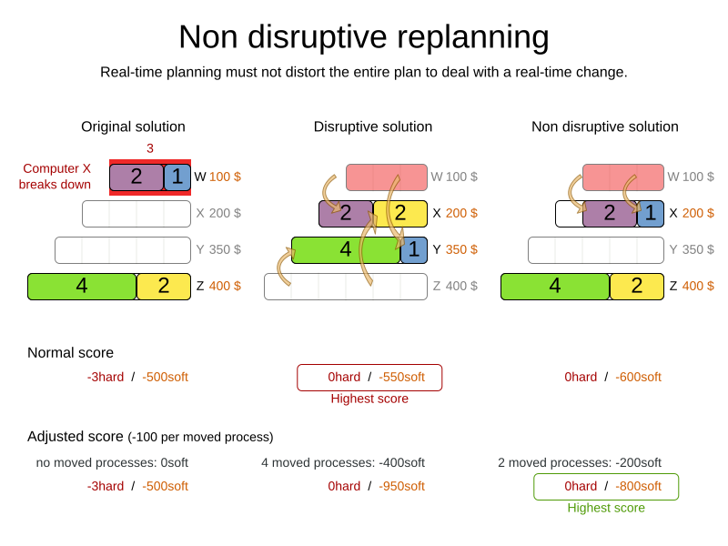
In the machine reassignment example, the entity has both the planning variable machine and its original value original_machine:
from optapy import planning_entity, planning_variable

@planning_entity(...)
class ProcessAssignment:
    process: MrProcess
    original_machine: Machine
    machine: Machine

    @planning_variable(...)
    def get_machine(self) -> Machine:
        ...

    def is_moved(self) -> bool:
        return (self.original_machine is not None and
                self.original_machine != self.machine)
    ...
During planning, the planning variable machine changes.
By comparing it with the originalMachine, a change in plan can be penalized:
from optapy import get_class
from optapy.constraint import ConstraintFactory, Constraint

ProcessAssignmentClass = get_class(ProcessAssignment)

def process_moved(constraint_factory: ConstraintFactory):
    return constraint_factory.forEach(ProcessAssignmentClass) \
               .filter(lambda process_assignment: process_assignment.is_moved()) \
               .penalize("process_moved", HardSoftScore.ofSoft(1000))
The soft penalty of -1000 means that a better solution is only accepted if it improves the soft score for at least 1000 points per variable changed (or if it improves the hard score).
5. Real-time planning
To do real-time planning, combine the following planning techniques:
-
Backup planning - adding extra score constraints to allow for unforeseen changes.
-
Continuous planning - planning for one or more future planning periods.
-
Short planning windows.
This lowers the burden of real-time planning.
As time passes, the problem itself changes. Consider the vehicle routing use case:
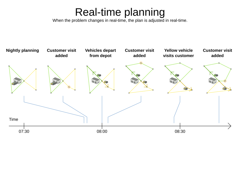
In the example above, three customers are added at different times (07:56, 08:02 and 08:45), after the original customer set finished solving at 07:55, and in some cases, after the vehicles have already left.
OptaPlanner can handle such scenarios with ProblemChange (in combination with pinned planning entities).
5.1. ProblemChange
While the Solver is solving, one of the problem facts may be changed by an outside event.
For example, an airplane is delayed and needs the runway at a later time.
|
Do not change the problem fact instances used by the |
Add a ProblemChange to the Solver, which it executes in the solver thread as soon as possible.
For example:
class Solver:
    # ...
    def addProblemChange(self, problem_change: Callable[[Solution, ProblemChangeDirector], None]) -> None:
        ...
    def isEveryProblemChangeProcessed(self) -> bool:
        ...
    ...
Similarly, you can pass the ProblemChange to the SolverManager:
class SolverManager:
    # ...
    def addProblemChange(self, problem_id: ProblemId, problem_change: ProblemChange) -> CompletableFuture[None]:
        ...
    ...
and the SolverJob:
class SolverJob:
    # ...
    def addProblemChange(self, problem_change: ProblemChange) -> CompletableFuture[None]:
        ...
    ...
Notice the method returns CompletableFuture[None], which is completed when a user-defined Consumer accepts
the best solution containing this problem change.
class ProblemChange:
    def doChange(self, working_solution: Solution, problem_change_director: ProblemChangeDirector) -> None:
        ...
...|
The |
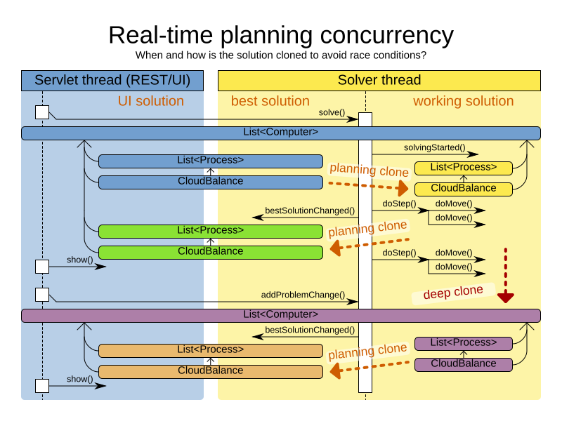
To write a ProblemChange correctly, it is important to understand the behavior of a planning clone.
A planning clone of a solution must fulfill these requirements:
-
The clone must represent the same planning problem. Usually it reuses the same instances of the problem facts and problem fact collections as the original.
-
The clone must use different, cloned instances of the entities and entity collections. Changes to an original Solution entity’s variables must not affect its clone.
5.1.1. Cloud balancing ProblemChange example
Consider the following example of a ProblemChange implementation in the cloud balancing use case:
from optapy import problem_change

@problem_change
class DeleteComputerProblemChange:
    def __init__(self, deleted_computer):
        self.deleted_computer = deleted_computer

    def doChange(self, cloud_balance, problem_change_director):
        working_computer = problem_change_director.lookUpWorkingObject(self.deleted_computer);
        if working_computer is None:
            raise ValueError(f"A computer ({self.deleted_computer} does not exist. Maybe it has been already deleted.")
        # First remove the problem fact from all planning entities that use it
        for process in cloud_balance.process_list:
            if process.computer == working_computer:
                problem_change_director.changeVariable(process, "computer",
                        lambda working_process: working_process.set_computer(None))
        # A SolutionCloner does not clone problem fact lists (such as computer_list)
        # Shallow clone the computer_list so only working_solution is affected, not best_solution or gui_solution
        computer_list = cloud_balance.computer_list.copy()
        cloud_balance.computer_list =computer_list
        # Remove the problem fact itself
        problem_change_director.removeProblemFact(working_computer, lambda working_computer_list: working_computer_list.remove(self.deleted_computer))

def delete_computer(computer: CloudComputer) -> None:
solver.addProblemChange(DeleteComputerProblemChange(computer))-
Any change in a
@problem_changemust be done on theworking_solution(the first parameter in thedoChangemethod). -
The
working_solutionis a planning clone of theBestSolutionChangedEvent'sbest_solution.-
The
working_solutionin theSolveris never the same solution instance as in the rest of your application: it is a planning clone. -
A planning clone also clones the planning entities and planning entity collections.
Thus, any change on the planning entities must happen on the
working_solutioninstance passed to theProblemChange.doChange(working_solution: Solution, problem_change_director: ProblemChangeDirector)method.
-
-
Use the method
ProblemChangeDirector.lookUpWorkingObject()to translate and retrieve the working solution’s instance of an object. This requires annotating a property of that class as the @planning_id. -
A planning clone does not clone the problem facts, nor the problem fact collections. Therefore the
working_solutionand thebest_solutionshare the same problem fact instances and the same problem fact list instances.Any problem fact or problem fact list changed by a
ProblemChangemust be problem cloned first (which can imply rerouting references in other problem facts and planning entities). Otherwise, if theworking_solutionandbest_solutionare used in different threads (for example a solver thread and a GUI event thread), a race condition can occur.
5.1.2. Cloning solutions to avoid race conditions in real-time planning
Many types of changes can leave a planning entity uninitialized, resulting in a partially initialized solution. This is acceptable, provided the first solver phase can handle it.
All construction heuristics solver phases can handle a partially initialized solution, so it is recommended to configure such a solver phase as the first phase.
The process occurs as follows:
-
The
Solverstops. -
Runs the
ProblemChange. -
restarts.
This is a warm start because its initial solution is the adjusted best solution of the previous run.
-
Each solver phase runs again.
This implies the construction heuristic runs again, but because little or no planning variables are uninitialized (unless you have a nullable planning variable), it finishes much quicker than in a cold start.
-
Each configured
Terminationresets (both in solver and phase configuration), but a previous call toterminateEarly()is not undone.Terminationis not usually configured (except in daemon mode); instead,Solver.terminateEarly()is called when the results are needed. Alternatively, configure aTerminationand use the daemon mode in combination withBestSolutionChangedEventas described in the following section.
5.2. Daemon: solve() does not return
In real-time planning, it is often useful to have a solver thread wait when it runs out of work, and immediately resume solving a problem once new problem fact changes are added.
Putting the Solver in daemon mode has the following effects:
-
If the
Solver'sTerminationterminates, it does not return fromsolve(), but blocks its thread instead (which frees up CPU power).-
Except for
terminateEarly(), which does make it return fromsolve(), freeing up system resources and allowing an application to shutdown gracefully. -
If a
Solverstarts with an empty planning entity collection, it waits in the blocked state immediately.
-
-
If a
ProblemChangeis added, it goes into the running state, applies theProblemChangeand runs theSolveragain.
To use the Solver in daemon mode:
-
Enable
daemonmode on theSolver:<solver xmlns="https://www.optaplanner.org/xsd/solver" xmlns:xsi="http://www.w3.org/2001/XMLSchema-instance" xsi:schemaLocation="https://www.optaplanner.org/xsd/solver https://www.optaplanner.org/xsd/solver/solver.xsd"> <daemon>true</daemon> ... </solver>Do not forget to call
Solver.terminateEarly()when your application needs to shutdown to avoid killing the solver thread unnaturally. -
Subscribe to the
BestSolutionChangedEventto process new best solutions found by the solver thread.A
BestSolutionChangedEventdoes not guarantee that everyProblemChangehas been processed already, nor that the solution is initialized and feasible. -
To ignore
BestSolutionChangedEvents with such invalid solutions, do the following:def best_solution_changed(event: BestSolutionChangedEvent[CloudBalance]) -> None: if (event.isEveryProblemChangeProcessed() and # Ignore infeasible (including uninitialized) solutions event.getNewBestScore().isFeasible()): ... -
Use
Score.isSolutionInitialized()instead ofScore.isFeasible()to only ignore uninitialized solutions, but do accept infeasible solutions too.
6. Multi-stage planning
In multi-stage planning, complex planning problems are broken down in multiple stages. A typical example is train scheduling, where one department decides where and when a train will arrive or depart and another department assigns the operators to the actual train cars or locomotives.
Each stage has its own solver configuration (and therefore its own SolverFactory):
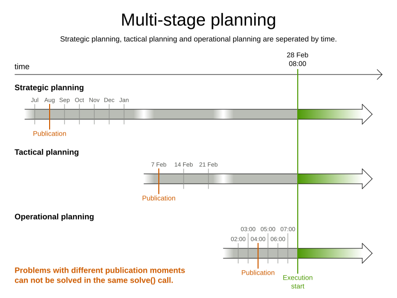
Planning problems with different publication deadlines must use multi-stage planning. But problems with the same publication deadline, solved by different organizational groups are also initially better off with multi-stage planning, because of Conway’s law and the high risk associated with unifying such groups.
Similarly to Partitioned Search, multi-stage planning leads to suboptimal results. Nevertheless, it might be beneficial in order to simplify the maintenance, ownership, and help to start a project.
Do not confuse multi-stage planning with multi-phase solving.