OptaPy configuration
1. Overview
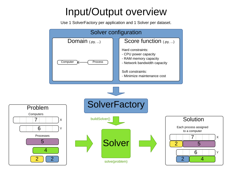
Solving a planning problem with OptaPy consists of the following steps:
-
Model your planning problem as a class annotated with the
@planning_solutiondecorator, for example theNQueensclass. -
Configure a
Solver, for example a First Fit and Tabu Search solver for anyNQueensinstance. -
Load a problem data set from your data layer, for example a Four Queens instance. That is the planning problem.
-
Solve it with
Solver.solve(problem)which returns the best solution found.
2. Solver configuration
2.1. Solver configuration by XML
Build a Solver instance with the SolverFactory.
Create a SolverFactory by passing a SolverConfig to
solver_factory_create.
A SolverConfig can be created from a XML file, like so:
from optapy import solver_config_create_from_xml_file
import pathlib

solver_config = solver_config_create_from_xml_file(pathlib.Path('solverConfig.xml'))

solver_factory = solver_factory_create(solver_config)

solver_factory.buildSolver().solve(generate_problem())
A solver configuration XML file looks like this:
<?xml version="1.0" encoding="UTF-8"?>
<solver xmlns="https://www.optaplanner.org/xsd/solver" xmlns:xsi="http://www.w3.org/2001/XMLSchema-instance"
    xsi:schemaLocation="https://www.optaplanner.org/xsd/solver https://www.optaplanner.org/xsd/solver/solver.xsd">
  <!-- Define the model -->
  <solutionClass>optapy.examples.domain.NQueens</solutionClass>
  <entityClass>optapy.examples.domain.Queen</entityClass>

  <!-- Define the score function -->
  <scoreDirectorFactory>
    <constraintProviderClass>optapy.examples.constraints.n_queens_constraints</constraintProviderClass>
  </scoreDirectorFactory>

  <!-- Configure the optimization algorithms (optional) -->
  <termination>
    ...
  </termination>
  <constructionHeuristic>
    ...
  </constructionHeuristic>
  <localSearch>
    ...
  </localSearch>
</solver>|
For XML elements that end in "Class" (solutionClass, entityClass, constraintProviderClass, etc.), put "{module}.{name}", where {module} is the module the class/function was defined in, and name is the name of the class/function. If the module is "__main__", put "{name}" instead. For instance, if the below code was in the main module: Use "my.domain.MyEntity" to refer to "MyEntity", "MySolution" to refer to "MySolution", and "my_constraints" to refer to "my_constraints". |
Notice the three parts in it:
-
Define the model.
-
Define the score function.
-
Optionally configure the optimization algorithm(s).
These various parts of a configuration are explained further in this manual.
OptaPy makes it relatively easy to switch optimization algorithm(s) just by changing the configuration.
2.2. Solver configuration by Python API
A solver configuration can also be configured with the SolverConfig API.
This is especially useful to change some values dynamically at runtime.
For example, to change the running time based on an environment variable, before building the Solver:
import os
import optapy
import optapy.config
import pathlib

SOLVE_TIME_IN_MINUTES = os.environ['SOLVE_TIME_IN_MINUTES']
termination_config = optapy.config.solver.TerminationConfig() \
    .withMinutesSpentLimit(SOLVE_TIME_IN_MINUTES)

solver_config = solver_config_create_from_xml_file(pathlib.Path('solverConfig.xml')) \
    .withTerminationConfig(termination_config)

solver_factory = solver_factory_create(solver_config)

solver_factory.buildSolver().solve(generate_problem())
Every element in the solver configuration XML is available as a *Config class
or a property on a *Config class in the package optapy.config.
These *Config classes are the Python representation of the XML format.
They build the runtime components and assemble them into an efficient Solver.
|
To configure a |
3. Model a planning problem
3.1. Is this class a problem fact or planning entity?
Look at a dataset of your planning problem. You will recognize domain classes in there, each of which can be categorized as one of the following:
-
An unrelated class: not used by any of the score constraints. From a planning standpoint, this data is obsolete.
-
A problem fact class: used by the score constraints, but does NOT change during planning (as long as the problem stays the same). For example:
Bed,Room,Shift,Employee,Topic,Period, … All the properties of a problem fact class are problem properties. -
A planning entity class: used by the score constraints and changes during planning. For example:
BedDesignation,ShiftAssignment,Exam, … The properties that change during planning are planning variables. The other properties are problem properties.
Ask yourself: What class changes during planning? Which class has variables that I want the Solver to change for me? That class is a planning entity.
Most use cases have only one planning entity class.
Most use cases also have only one planning variable per planning entity class.
In xref:repeated-planning/repeated-planning.adoc#realTimePlanning[real-time planning], even though the problem itself changes, problem facts do not really change during planning, instead they change between planning (because the Solver temporarily stops to apply the problem fact changes). |
To create a good domain model, read the domain modeling guide.
In OptaPy, all problem facts and planning entities are plain old Python Objects. Load them from a database, an XML file, a data repository, a REST service, a noSQL cloud; it doesn’t matter.
3.2. Problem fact
A problem fact is any Python Object with getters that does not change during planning. For example in n queens, the columns and rows are problem facts:
from optapy import problem_fact

@problem_fact
class Column:
    def __init__(self, index):
        self.index = index
    ...
from optapy import problem_fact
@problem_fact
class Row:
def __init__(self, index):
self.index = index
...A problem fact can reference other problem facts of course:
from optapy import problem_fact

@problem_fact
class Teacher:
    ...

@problem_fact
class Curriculum:
    ...

@problem_fact
class Course:
    code: str
    teacher: Teacher # Other problem fact
    lecture_size: int
    min_working_day_size: int
    curriculum_list: list[Curriculum] # Other problem facts
    student_size: int
    ...
Unlike OptaPlanner, a problem fact class must be decorated with @problem_fact to be used in constraints.
|
Generally, better designed domain classes lead to simpler and more efficient score constraints.
Therefore, when dealing with a messy (denormalized) legacy system, it can sometimes be worthwhile to convert the messy domain model into a OptaPy specific model first.
For example: if your domain model has two |
3.3. Planning entity
3.3.1. Planning entity decorator
A planning entity is a Python Object that changes during solving, for example a Queen that changes to another row.
A planning problem has multiple planning entities, for example for a single n queens problem, each Queen is a planning entity.
But there is usually only one planning entity class, for example the Queen class.
A planning entity class needs to be decorated with the @planning_entity decorator.
Each planning entity class has one or more planning variables (which can be genuine or shadows).
It should also have one or more defining properties.
For example in n queens, a Queen is defined by its Column and has a planning variable Row.
This means that a Queen’s column never changes during solving, while its row does change.
from optapy import planning_entity

@planning_entity
class Queen:
    column: Column

    # Planning variables: changes during planning, between score calculations.
    row: Row
    # ... getters and setters
A planning entity class can have multiple planning variables.
For example, a Lecture is defined by its Course and its index in that course (because one course has multiple lectures).
Each Lecture needs to be scheduled into a Period and a Room so it has two planning variables (period and room).
For example: the course Mathematics has eight lectures per week, of which the first lecture is Monday morning at 08:00 in room 212.
from optapy import planning_entity

@planning_entity
class Lecture:
    course: Course
    lectureIndexInCourse: int

    # Planning variables: changes during planning, between score calculations.
    period: Period
    room: Room
    ...
The solver configuration needs to declare each planning entity class:
<solver xmlns="https://www.optaplanner.org/xsd/solver" xmlns:xsi="http://www.w3.org/2001/XMLSchema-instance"
    xsi:schemaLocation="https://www.optaplanner.org/xsd/solver https://www.optaplanner.org/xsd/solver/solver.xsd">
  ...
  <entityClass>optapy.examples.domain.Queen</entityClass>
  ...
</solver>
Some uses cases have multiple planning entity classes. For example: route freight and trains into railway network arcs, where each freight can use multiple trains over its journey and each train can carry multiple freights per arc. Having multiple planning entity classes directly raises the implementation complexity of your use case.
|
Do not create unnecessary planning entity classes. This leads to difficult For example, do not create a planning entity class to hold the total free time of a teacher, which needs to be kept up to date as the If historic data needs to be considered too, then create problem fact to hold the total of the historic assignments up to, but not including, the planning window (so that it does not change when a planning entity changes) and let the score constraints take it into account. |
|
Planning entity |
3.4. Planning variable (genuine)
3.4.1. Planning variable decorator
A planning variable is a Python property (so a getter and setter) on a planning entity.
It points to a planning value, which changes during planning.
For example, a Queen's row property is a genuine planning variable.
Note that even though a Queen's row property changes to another Row during planning, no Row instance itself is changed.
Normally planning variables are genuine, but advanced cases can also have shadows.
A genuine planning variable getter needs to be annotated with the @planning_variable annotation, which needs a non-empty variable_type and value_range_provider_refs property.
from optapy import planning_entity, planning_variable

@planning_entity
class Queen:
    # ...
    row: Row

    # Alternatively, @planning_variable(Row, ["row_range"])
    @planning_variable(variable_type = Row, value_range_provider_refs = ["row_range"])
    def get_row(self):
        return self.row

    def set_row(self, row):
        self.row = row
The variable_type property define the type of planning values this planning variable takes. The variable_type does not need to be decorated with @problem_fact; it can be any Python type.
The value_range_provider_refs property defines what are the possible planning values for this planning variable.
It references one or more @ValueRangeProvider id's.
3.4.2. Nullable planning variable
By default, an initialized planning variable cannot be None, so an initialized solution will never use None for any of its planning variables.
In an over-constrained use case, this can be counterproductive.
For example: in task assignment with too many tasks for the workforce, we would rather leave low priority tasks unassigned instead of assigning them to an overloaded worker.
To allow an initialized planning variable to be None, set nullable to True:
    @planning_variable(..., nullable = True)
    def get_worker(self):
return self.worker|
Constraint Streams filter out planning entities with a |
OptaPy will automatically add the value None to the value range.
There is no need to add None in a collection provided by a @value_range_provider.
|
Using a nullable planning variable implies that your score calculation is responsible for punishing (or even rewarding) variables with a |
|
Currently chained planning variables are not compatible with |
Repeated planning (especially real-time planning) does not mix well with a nullable planning variable.
Every time the Solver starts or a problem fact change is made, the Construction Heuristics
will try to initialize all the None variables again, which can be a huge waste of time.
One way to deal with this is to filter the entity selector of the placer in the construction heuristic.
<solver xmlns="https://www.optaplanner.org/xsd/solver" xmlns:xsi="http://www.w3.org/2001/XMLSchema-instance"
    xsi:schemaLocation="https://www.optaplanner.org/xsd/solver https://www.optaplanner.org/xsd/solver/solver.xsd">
  ...
  <constructionHeuristic>
    <queuedEntityPlacer>
      <entitySelector id="entitySelector1">
        <filterClass>...</filterClass>
      </entitySelector>
    </queuedEntityPlacer>
    ...
    <changeMoveSelector>
      <entitySelector mimicSelectorRef="entitySelector1" />
    </changeMoveSelector>
    ...
  </constructionHeuristic>
 ...
</solver>
3.4.3. When is a planning variable considered initialized?
A planning variable is considered initialized if its value is not None or if the variable is nullable.
So a nullable variable is always considered initialized.
A planning entity is initialized if all of its planning variables are initialized.
A solution is initialized if all of its planning entities are initialized.
3.4.4. Planning value
A planning value is a possible value for a genuine planning variable.
Usually, a planning value is a problem fact, but it can also be any object, for example an int.
It can even be another planning entity or even an interface implemented by both a planning entity and a problem fact.
A planning value range is the set of possible planning values for a planning variable.
This set can be a countable (for example row 1, 2, 3 or 4) or uncountable (for example any float between 0.0 and 1.0).
3.4.5. Planning value range provider
Overview
The value range of a planning variable is defined with the @value_range_provider decorator.
A @value_range_provider decorator always has a property range_id, which is referenced by the @planning_variable's property value_range_provider_refs.
This annotation can be located on two types of methods:
-
On the Solution: All planning entities share the same value range.
-
On the planning entity: The value range differs per planning entity. This is less common.
|
A @value_range_provider annotation needs to be on a member in a class with a |
The return type of that method can be two types:
-
List: The value range is defined by a list of its possible values. -
ValueRange: The value range is defined by its bounds. This is less common.
ValueRangeProvider on the solution
All instances of the same planning entity class share the same set of possible planning values for that planning variable. This is the most common way to configure a value range.
The @planning_solution implementation has method that returns a list (or a ValueRange).
Any value from that list is a possible planning value for this planning variable.
    @planning_variable(Row, value_range_provider_refs = {"row_range"})
    def get_row(self):
        return self.row
from optapy import planning_solution, value_range_provider, problem_fact_collection_property
@planning_solution
class NQueens:
# ...
@value_range_provider(range_id = "row_range")
def get_row_list(self):
return self.row_list|
That |
ValueRangeProvider on the Planning Entity
Each planning entity has its own value range (a set of possible planning values) for the planning variable. For example, if a teacher can never teach in a room that does not belong to his department, lectures of that teacher can limit their room value range to the rooms of his department.
    @planning_variable(Room, value_range_provider_refs = ["department_room_range"])
    def get_room(self):
        return self.room

    @value_range_provider(range_id = "department_room_range", value_range_type = Room)
    def get_possible_room_list(self):
        return self.course.teacher.department.room_list
Never use this to enforce a soft constraint (or even a hard constraint when the problem might not have a feasible solution). For example: Unless there is no other way, a teacher cannot teach in a room that does not belong to his department. In this case, the teacher should not be limited in his room value range (because sometimes there is no other way).
|
By limiting the value range specifically of one planning entity, you are effectively creating a built-in hard constraint. This can have the benefit of severely lowering the number of possible solutions; however, it can also take away the freedom of the optimization algorithms to temporarily break that constraint in order to escape from a local optimum. |
A planning entity should not use other planning entities to determine its value range. That would only try to make the planning entity solve the planning problem itself and interfere with the optimization algorithms.
Every entity has its own list instance, unless multiple entities have the same value range.
For example, if teacher A and B belong to the same department, they use the same list instance.
Furthermore, each list contains a subset of the same set of planning value instances.
For example, if department A and B can both use room X, then their list instances contain the same Room instance.
|
A |
|
A |
ValueRangeFactory
Instead of a Collection, you can also return a ValueRange or CountableValueRange, built by the ValueRangeFactory:
from optapy import planning_solution, value_range_provider
from optapy.types import CountableValueRange, ValueRangeFactory

    @value_range_provider(range_id = "delay_range", value_range_type = CountableValueRange)
    def get_delay_range(self):
        return ValueRangeFactory.createIntValueRange(0, 5000)
A ValueRange uses far less memory, because it only holds the bounds.
In the example above, a list would need to hold all 5000 ints, instead of just the two bounds.
Furthermore, an incrementUnit can be specified, for example if you have to buy stocks in units of 200 pieces:
from optapy import planning_solution, value_range_provider
from optapy.types import CountableValueRange, ValueRangeFactory

    @value_range_provider(range_id = "stock_amount_range", value_range_type = CountableValueRange)
    def get_stock_amount_range(self) {
        # Range: 0, 200, 400, 600, ..., 9999600, 9999800, 10000000
        return ValueRangeFactory.createIntValueRange(0, 10000000, 200)
}|
Return |
The ValueRangeFactory has creation methods for several value class types:
-
boolean: A boolean range. -
int: A 32bit integer range. -
long: A 64bit integer range. -
double: A 64bit floating point range which only supports random selection (because it does not implementCountableValueRange). -
BigInteger: An arbitrary-precision integer range. -
BigDecimal: A decimal point range. By default, the increment unit is the lowest non-zero value in the scale of the bounds. -
Temporal(such asLocalDate,LocalDateTime, …): A time range.
Combine ValueRangeProviders
Value range providers can be combined, for example:
    @planning_variable(value_range_provider_refs = ["company_car_range", "personal_car_range"])
    def get_car(self):
        return self.car
    }
@value_range_provider(id = "company_car_range")
def get_company_car_list(self):
return self.company_car_list
@value_range_provider(id = "personal_car_range")
def get_personal_car_list(self):
return self.personal_car_list3.4.6. Planning value strength
Planning value difficulty is not yet supported, but will be in a future version.
3.4.7. Planning List Variable
In some use cases, such as Vehicle Routing and Task Assignment, it is more convenient to model the planning variables as a list. For example, the list of customers a vehicle visits, or the list of tasks a person does. In OptaPy, this is accomplished by using planning list variables.
For a planning list variable with value range "value_range":
-
The order of elements inside the list is significant
-
All values in "value_range" appear in exactly one planning entity’s planning list variable
To declare a planning list variable, use the @planning_list_variable decorator:
from optapy import planning_entity, planning_list_variable

@planning_entity
class Vehicle:
    def __init__(self, _id, capacity, depot, customer_list=None):
        self.id = _id
        self.capacity = capacity
        self.depot = depot
        if customer_list is None:
            self.customer_list = []
        else:
            self.customer_list = customer_list

    @planning_list_variable(Customer, ['customer_range'])
    def get_customer_list(self):
        return self.customer_list

...|
The getter for |
3.4.8. Chained planning variable (TSP, VRP, …)
Some use cases, such as TSP and Vehicle Routing, require chaining. This means the planning entities point to each other and form a chain. By modeling the problem as a set of chains (instead of a set of trees/loops), the search space is heavily reduced.
|
Planning list variables can also be used for these use cases |
A planning variable that is chained either:
-
Directly points to a problem fact (or planning entity), which is called an anchor.
-
Points to another planning entity with the same planning variable, which recursively points to an anchor.
Here are some examples of valid and invalid chains:
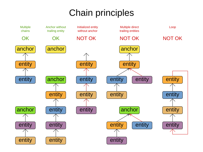
Every initialized planning entity is part of an open-ended chain that begins from an anchor. A valid model means that:
-
A chain is never a loop. The tail is always open.
-
Every chain always has exactly one anchor. The anchor is never an instance of the planning entity class that contains the chained planning variable.
-
A chain is never a tree, it is always a line. Every anchor or planning entity has at most one trailing planning entity.
-
Every initialized planning entity is part of a chain.
-
An anchor with no planning entities pointing to it, is also considered a chain.
|
A planning problem instance given to the |
|
If your constraints dictate a closed chain, model it as an open-ended chain (which is easier to persist in a database) and implement a score constraint for the last entity back to the anchor. |
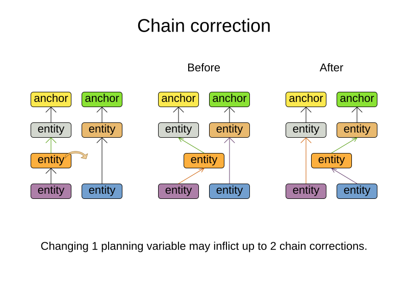
The optimization algorithms and built-in Moves do chain correction to guarantee that the model stays valid:
|
A custom |
For example, in TSP the anchor is a Domicile (in vehicle routing it is Vehicle):
from optapy import problem_fact, planning_entity, planning_variable
from optapy.types import PlanningVariableGraphType

@problem_fact
class Standstill:
    def get_city(self):
        raise NotImplementedError()


@problem_fact
class Domicile(Standstill):
    # ...
    def get_city(self):
        return self.city


@planning_entity
class Visit(Standstill):
    # ...
    @planning_variable(Standstill, value_range_provider_refs=['domicile_range', 'visit_range'],
                              graph_type=PlanningVariableGraphType.CHAINED)
    def get_previous_standstill(self):
        return self.previous_standstill

    def set_previous_standstill(self, previous_standstill):
        self.previous_standstill = previous_standstill
Notice how two value range providers are usually combined:
-
The value range provider that holds the anchors, for example
domicile_list. -
The value range provider that holds the initialized planning entities, for example
visit_list.
3.5. Planning problem and planning solution
3.5.1. Planning problem instance
A dataset for a planning problem needs to be wrapped in a class for the Solver to solve.
That solution class represents both the planning problem and (if solved) a solution.
It is decorated with a @planning_solution decorator.
For example in n queens, the solution class is the NQueens class, which contains a Column list, a Row list, and a Queen list.
A planning problem is actually an unsolved planning solution or - stated differently - an uninitialized solution.
For example in n queens, that NQueens class has the @planning_solution annotation, yet every Queen in an unsolved NQueens class is not yet assigned to a Row (their row property is null). That’s not a feasible solution.
It’s not even a possible solution.
It’s an uninitialized solution.
3.5.2. Solution class
A solution class holds all problem facts, planning entities and a score.
It is annotated with a @PlanningSolution annotation.
For example, an NQueens instance holds a list of all columns, all rows and all Queen instances:
from optapy import planning_solution
from optapy.score import SimpleScore

@planning_solution
class NQueens:
    # Problem facts
    n: int
    column_list: list[Column]
    row_list: list[Row]

    # Planning entities
    queen_list: list[Queen]

    score: SimpleScore
    ...
The solver configuration needs to declare the planning solution class:
<solver xmlns="https://www.optaplanner.org/xsd/solver" xmlns:xsi="http://www.w3.org/2001/XMLSchema-instance"
    xsi:schemaLocation="https://www.optaplanner.org/xsd/solver https://www.optaplanner.org/xsd/solver/solver.xsd">
  ...
  <solutionClass>optapy.examples.domain.NQueens</solutionClass>
  ...
</solver>
3.5.3. Planning entities of a solution (@planning_entity_collection_property)
OptaPy needs to extract the entity instances from the solution instance.
It gets those collection(s) by calling every getter that is annotated with @planning_entity_collection_property:
from optapy import planning_solution, planning_entity_collection_property

@planning_solution
class NQueens :
    # ...
    queen_list: list[Queen]

    @planning_entity_collection_property(Queen)
    def get_queen_list(self):
        return self.queen_list
There can be multiple @planning_entity_collection_property decorated getters.
Those can even return a list with the same entity class type.
|
A |
In rare cases, a planning entity might be a singleton: use planning_entity_property on its getter instead.
3.5.4. Score of a Solution (@PlanningScore)
A @planning_solution class requires a score property (or field), which is annotated with a @planning_score annotation.
The score property is None if the score hasn’t been calculated yet.
The score property is typed to the specific Score implementation of your use case.
For example, NQueens uses a SimpleScore:
from optapy import planning_solution, planning_score
from optapy.score import SimpleScore

@planning_solution
class NQueens:
    # ...
    score: SimpleScore

    @planning_score(SimpleScore)
    def get_score(self):
        return self.score

    def set_score(self, score):
        self.score = score
Most use cases use a HardSoftScore instead:
@planning_solution
class CloudBalance:
    # ...
    score: HardSoftScore

    @planning_score(HardSoftScore)
    def get_score(self):
        return self.score

    def set_score(self, score):
        self.score = score
Some use cases use other score types.
3.5.5. Problem facts of a solution (@problem_fact_collection_property)
For Constraint Streams score calculation,
OptaPlanner needs to extract the problem fact instances from the solution instance.
It gets those collection(s) by calling every method (or field) that is annotated with @problem_fact_collection_property.
All objects returned by those methods are available to use by Constraint Streams.
For example in NQueens all Column and Row instances are problem facts.
from optapy import planning_solution, problem_fact_collection_property

@planning_solution
class NQueens:
    # ...

    column_list: list[Column]
    row_list: list[Row]

    @problem_fact_collection_property(Column)
    def get_column_list(self):
        return self.column_list

    @problem_fact_collection_property(Row)
    def get_row_list(self):
        return self.row_list
All planning entities are automatically inserted into the working memory.
Do not add @problem_fact_collection_property on their properties.
|
The problem facts methods are not called often: at most only once per solver phase per solver thread. |
There can be multiple @problem_fact_collection_property annotated members.
Those can even return a list with the same class type, but they shouldn’t return the same instance twice.
|
A |
In rare cases, a problem fact might be a singleton: use @problem_fact_property on its method instead.
Cached problem fact
A cached problem fact is a problem fact that does not exist in the real domain model, but is calculated before the Solver really starts solving.
The problem facts methods have the opportunity to enrich the domain model with such cached problem facts, which can lead to simpler and faster score constraints.
For example in examination, a cached problem fact TopicConflict is created for every two Topics which share at least one Student.
    @problem_fact_collection_property(TopicConflict)
    def calculate_topic_conflict_list(self): list[TopicConflict]:
        topic_conflict_list = []
        for left_topic in self.topic_list:
            for right_topic in self.topic_list:
                if left_topic.topic_id < right_topic.topic_id:
                    student_size = 0
                    for student in left_topic.student_list:
                        if student in right_topic.student_list:
                            student_size += 1
                    if student_size > 0:
                        topic_conflict_list.append(TopicConflict(left_topic, right_topic, student_size))
        return topic_conflict_list
Where a score constraint needs to check that no two exams with a topic that shares a student are scheduled close together (depending on the constraint: at the same time, in a row, or in the same day), the TopicConflict instance can be used as a problem fact, rather than having to combine every two Student instances.
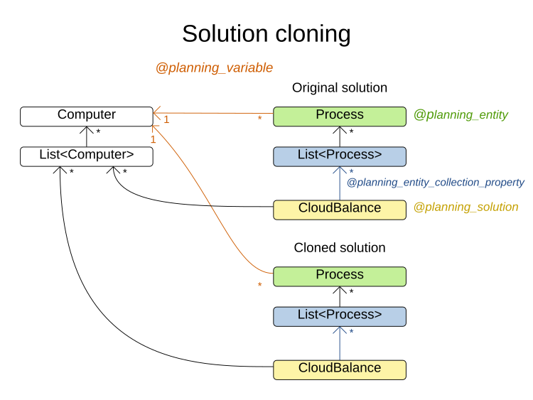
3.5.6. Cloning a solution
Most (if not all) optimization algorithms clone the solution each time they encounter a new best solution (so they can recall it later) or to work with multiple solutions in parallel.
|
There are many ways to clone, such as a shallow clone, deep clone, … This context focuses on a planning clone. |
A planning clone of a solution must fulfill these requirements:
-
The clone must represent the same planning problem. Usually it reuses the same instances of the problem facts and problem fact collections as the original.
-
The clone must use different, cloned instances of the entities and entity collections. Changes to an original solution entity’s variables must not affect its clone.
Implementing a planning clone method is hard, therefore you do not need to implement it.
FieldAccessingSolutionCloner
This SolutionCloner is used by default.
It works well for most use cases.
|
When the |
The FieldAccessingSolutionCloner does not clone problem facts by default.
If any of your problem facts needs to be deep cloned for a planning clone,
for example if the problem fact references a planning entity or the planning solution,
mark its class with a @deep_planning_clone decorator:
from optapy import problem_fact, deep_planning_clone

@problem_fact
@deep_planning_clone
class SeatDesignationDependency:
    left_seat_designation: SeatDesignation # planning entity
    right_seat_designation: SeatDesignation # planning entity
    ...
In the example above, because SeatDesignationDependency references the planning entity SeatDesignation
(which is deep planning cloned automatically), it should also be deep planning cloned.
Alternatively, the @deep_planning_clone decorator also works on a getter method to planning clone it.
If that property is a list or a map, it will shallow clone it and deep planning clone
any element thereof that is an instance of a class that has a @deep_planning_clone decorator.
3.5.7. Create an uninitialized solution
Create a @planning_solution class instance to represent your planning problem’s dataset, so it can be set on the Solver as the planning problem to solve.
For example in n queens, an NQueens instance is created with the required Column and Row instances and every Queen set to a different column and every row set to null.
    def create_n_queens(n: int) -> NQueens:
        n_queens = NQueens()
        n_queens.n = n
        n_queens.column_list = create_column_list(n_queens)
        n_queens.row_list = create_row_list(n_queens)
        n_queens.queen_list = create_queen_list(n_queens)
        return n_queens

    def create_queen_list(n_queens: NQueens) -> list[Queen]:
        n = n_queens.n
        queen_list = []
        queen_id = 0
        for column in n_queens.column_list:
            queen = Queen()
            queen.queen_id = id
            queen_id += 1
            queen.column = column
            # Notice that we leave the PlanningVariable properties as None
            queen_list.append(queen)
        return queen_list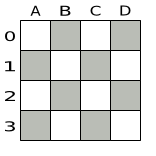
Usually, most of this data comes from your data layer, and your solution implementation just aggregates that data and creates the uninitialized planning entity instances to plan:
def create_lecture_list(schedule: CourseSchedule):
    course_list = schedule.course_list
    lecture_list = []
    lecture_id = 0
    for course in course_list:
        for i in range(course.lecture_size):
            lecture = Lecture()
            lecture.lecture_id = lecture_id
            lecture_id += 1
            lecture.course = course
            lecture.lecture_index_in_course = i
            # Notice that we leave the PlanningVariable properties (period and room) as None
            lecture_list.append(lecture)
    schedule.lecture_list = lecture_list
4. Use the Solver
4.1. The Solver interface
A Solver solves your planning problem.
A Solver can only solve one planning problem instance at a time.
It is built with a SolverFactory, there is no need to implement it yourself.
A Solver should only be accessed from a single thread, except for the methods that are specifically documented in javadoc as being thread-safe.
The solve() method hogs the current thread.
This can cause HTTP timeouts for REST services and it requires extra code to solve multiple datasets in parallel.
To avoid such issues, use a SolverManager instead.
4.2. Solving a problem
Solving a problem is quite easy once you have:
-
A
Solverbuilt from a solver configuration -
A
@planning_solutionthat represents the planning problem instance
Just provide the planning problem as argument to the solve() method and it will return the best solution found:
problem = ...
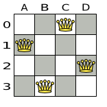
best_solution = solver.solve(problem)For example in n queens, the solve() method will return an NQueens instance with every Queen assigned to a Row.
The solve(Solution) method can take a long time (depending on the problem size and the solver configuration). The Solver intelligently wades through the search space of possible solutions and remembers the best solution it encounters during solving.
Depending on a number of factors (including problem size, how much time the Solver has, the solver configuration, …), that best solution might or might not be an optimal solution.
|
The solution instance given to the method The solution instance returned by the methods |
|
The solution instance given to the |
4.3. Environment mode: are there bugs in my code?
The environment mode allows you to detect common bugs in your implementation. It does not affect the logging level.
You can set the environment mode in the solver configuration XML file:
<solver xmlns="https://www.optaplanner.org/xsd/solver" xmlns:xsi="http://www.w3.org/2001/XMLSchema-instance"
    xsi:schemaLocation="https://www.optaplanner.org/xsd/solver https://www.optaplanner.org/xsd/solver/solver.xsd">
  <environmentMode>FAST_ASSERT</environmentMode>
  ...
</solver>
A solver has a single Random instance.
Some solver configurations use the Random instance a lot more than others.
For example, Simulated Annealing depends highly on random numbers, while Tabu Search only depends on it to deal with score ties.
The environment mode influences the seed of that Random instance.
These are the environment modes:
4.3.1. FULL_ASSERT
The FULL_ASSERT mode turns on all assertions (such as assert that the incremental score calculation is uncorrupted for each move) to fail-fast on a bug in a Move implementation, a constraint, the engine itself, …
This mode is reproducible (see the reproducible mode). It is also intrusive because it calls the method calculateScore() more frequently than a non-assert mode.
The FULL_ASSERT mode is horribly slow (because it does not rely on incremental score calculation).
4.3.2. NON_INTRUSIVE_FULL_ASSERT
The NON_INTRUSIVE_FULL_ASSERT turns on several assertions to fail-fast on a bug in a Move implementation, a constraint, the engine itself, …
This mode is reproducible (see the reproducible mode). It is non-intrusive because it does not call the method calculateScore() more frequently than a non assert mode.
The NON_INTRUSIVE_FULL_ASSERT mode is horribly slow (because it does not rely on incremental score calculation).
4.3.3. FAST_ASSERT
The FAST_ASSERT mode turns on most assertions (such as assert that an undoMove’s score is the same as before the Move) to fail-fast on a bug in a Move implementation, a constraint, the engine itself, …
This mode is reproducible (see the reproducible mode). It is also intrusive because it calls the method calculateScore() more frequently than a non assert mode.
The FAST_ASSERT mode is slow.
It is recommended to write a test case that does a short run of your planning problem with the FAST_ASSERT mode on.
4.3.4. REPRODUCIBLE (default)
The reproducible mode is the default mode because it is recommended during development. In this mode, two runs in the same OptaPlanner version will execute the same code in the same order. Those two runs will have the same result at every step, except if the note below applies. This enables you to reproduce bugs consistently. It also allows you to benchmark certain refactorings (such as a score constraint performance optimization) fairly across runs.
|
Despite the reproducible mode, your application might still not be fully reproducible because of:
|
The reproducible mode can be slightly slower than the non-reproducible mode. If your production environment can benefit from reproducibility, use this mode in production.
In practice, this mode uses the default, fixed random seed if no seed is specified, and it also disables certain concurrency optimizations (such as work stealing).
4.3.5. NON_REPRODUCIBLE
The non-reproducible mode can be slightly faster than the reproducible mode. Avoid using it during development as it makes debugging and bug fixing painful. If your production environment doesn’t care about reproducibility, use this mode in production.
In practice, this mode uses no fixed random seed if no seed is specified.
4.4. Logging level: what is the Solver doing?
The best way to illuminate the black box that is a Solver, is to play with the logging level:
-
error: Log errors, except those that are thrown to the calling code as a
RuntimeException.If an error happens, OptaPy normally fails fast. It does not log it as an error itself to avoid duplicate log messages. Meanwhile, the code is disrupted from doing further harm or obfuscating the error.
-
warn: Log suspicious circumstances.
-
info: Log every phase and the solver itself. See scope overview.
-
debug: Log every step of every phase. See scope overview.
-
trace: Log every move of every step of every phase. See scope overview.
|
Turning on Even Both cause congestion in multithreaded solving with most appenders, see below.. |
For example, set it to debug logging, to see when the phases end and how fast steps are taken:
INFO  Solving started: time spent (3), best score (-4init/0), random (JDK with seed 0).
DEBUG     CH step (0), time spent (5), score (-3init/0), selected move count (1), picked move (Queen-2 {null -> Row-0}).
DEBUG     CH step (1), time spent (7), score (-2init/0), selected move count (3), picked move (Queen-1 {null -> Row-2}).
DEBUG     CH step (2), time spent (10), score (-1init/0), selected move count (4), picked move (Queen-3 {null -> Row-3}).
DEBUG     CH step (3), time spent (12), score (-1), selected move count (4), picked move (Queen-0 {null -> Row-1}).
INFO  Construction Heuristic phase (0) ended: time spent (12), best score (-1), score calculation speed (9000/sec), step total (4).
DEBUG     LS step (0), time spent (19), score (-1),     best score (-1), accepted/selected move count (12/12), picked move (Queen-1 {Row-2 -> Row-3}).
DEBUG     LS step (1), time spent (24), score (0), new best score (0), accepted/selected move count (9/12), picked move (Queen-3 {Row-3 -> Row-2}).
INFO  Local Search phase (1) ended: time spent (24), best score (0), score calculation speed (4000/sec), step total (2).
INFO  Solving ended: time spent (24), best score (0), score calculation speed (7000/sec), phase total (2), environment mode (REPRODUCIBLE).
All time spent values are in milliseconds.
Configure the logging level by explicitly calling logging.getLogger('optapy').setLevel(logging.LEVEL):
import logging

logging.getLogger('optapy').setLevel(logging.DEBUG)
By default, INFO logging is used.
4.6. Random number generator
Many heuristics and metaheuristics depend on a pseudorandom number generator for move selection, to resolve score ties, probability based move acceptance, … During solving, the same Random instance is reused to improve reproducibility, performance and uniform distribution of random values.
To change the random seed of that Random instance, specify a randomSeed:
<solver xmlns="https://www.optaplanner.org/xsd/solver" xmlns:xsi="http://www.w3.org/2001/XMLSchema-instance"
    xsi:schemaLocation="https://www.optaplanner.org/xsd/solver https://www.optaplanner.org/xsd/solver/solver.xsd">
  <randomSeed>0</randomSeed>
  ...
</solver>
To change the pseudorandom number generator implementation, specify a randomType:
<solver xmlns="https://www.optaplanner.org/xsd/solver" xmlns:xsi="http://www.w3.org/2001/XMLSchema-instance"
    xsi:schemaLocation="https://www.optaplanner.org/xsd/solver https://www.optaplanner.org/xsd/solver/solver.xsd">
  <randomType>MERSENNE_TWISTER</randomType>
  ...
</solver>
The following types are supported:
-
JDK(default): Standard implementation (java.util.Random). -
MERSENNE_TWISTER: Implementation by Commons Math. -
WELL512A,WELL1024A,WELL19937A,WELL19937C,WELL44497AandWELL44497B: Implementation by Commons Math.
For most use cases, the randomType has no significant impact on the average quality of the best solution on multiple datasets.
5. SolverManager
A SolverManager is a facade for one or more Solver instances
to simplify solving planning problems in REST and other enterprise services.
Unlike the Solver.solve(…) method:
-
SolverManager.solve(…)returns immediately: it schedules a problem for asynchronous solving without blocking the calling thread. This avoids timeout issues of HTTP and other technologies. -
SolverManager.solve(…)solves multiple planning problems of the same domain, in parallel.
Internally a SolverManager manages a thread pool of solver threads, which call Solver.solve(…),
and a thread pool of consumer threads, which handle best solution changed events.
Build a SolverManager instance with the solver_manager_create(…) method:
from optapy import solver_manager_create, solver_config_create_from_xml_file
from optapy.types import Duration

solver_config = solver_config_create_from_xml_file("solverConfig.xml")
solver_manager = solver_manager_create(solver_config)
Each problem submitted to the SolverManager.solve(…) methods needs a unique problem ID.
Later calls to getSolverStatus(problemId) or terminateEarly(problemId) use that problem ID
to distinguish between the planning problems.
The problem ID must be an immutable class, such as int, str or uuid.
To retrieve the best solution, after solving terminates normally, use SolverJob.getFinalBestSolution():
import uuid

problem1 = ...
problem_id = uuid.uuid4()
# Returns immediately
solver_job = solver_manager.solve(problem_id, problem1)
...
solution1 = solver_job.getFinalBestSolution()
However, there are better approaches, both for solving batch problems before an end-user needs the solution as well as for live solving while an end-user is actively waiting for the solution, as explained below.
The current SolverManager implementation runs on a single computer node,
but future work aims to distribute solver loads across a cloud.
5.1. Solve batch problems
At night, batch solving is a great approach to deliver solid plans by breakfast, because:
-
There are typically few or no problem changes in the middle of the night. Some organizations even enforce a deadline, for example, submit all day off requests before midnight.
-
The solvers can run for much longer, often hours, because nobody’s waiting for it and CPU resources are often cheaper.
To solve a multiple datasets in parallel (limited by parallelSolverCount),
call solve(…) for each dataset:
from optapy.types import SolverManager

class TimeTableService:
    solver_manager: SolverManager

    # Returns immediately, call it for every dataset
    def solve_batch(self, time_table_id: int):
        solver_manager.solve(time_table_id,
                # Called once, when solving starts
                lambda the_id: self.find_by_id(the_id),
                # Called once, when solving ends
                lambda solution: self.save(solution))

    def find_by_id(self, time_table_id: int) -> TimeTable:
        ...

    def save(self, time_table: TimeTable) -> None:
        ...
A solid plan delivered by breakfast is great, even if you need to react on problem changes during the day.
5.2. Solve and listen to show progress to the end-user
When a solver is running while an end-user is waiting for that solution, the user might need to wait for several minutes or hours before receiving a result. To assure the user that everything is going well, show progress by displaying the best solution and best score attained so far.
To handle intermediate best solutions, use solveAndListen(…):
from optapy.types import SolverManager

class TimeTableService:
    solver_manager: SolverManager

    # Returns immediately
    def solve_live(self, time_table_id: int) -> None:
        solver_manager.solveAndListen(time_table_id,
                # Called once, when solving starts
                lambda the_id: self.find_by_id(time_table_id),
                # Called multiple times, for every best solution change
                lambda solution: self.save(solution))

    def find_by_id(self, time_table_id: int):
        ...

    def save(self, time_table: TimeTable) -> None:
        ...

    def stop_solving(self, time_table_id: int):
        solver_manager.terminateEarly(time_table_id)
This implementation is using the database to communicate with the UI, which polls the database. More advanced implementations push the best solutions directly to the UI or a messaging queue.
If the user is satisfied with the intermediate best solution
and does not want to wait any longer for a better one, call SolverManager.terminateEarly(problemId).