Design patterns
1. Design patterns introduction
OptaPy design patterns are generic reusable solutions to common challenges in the model or architecture of projects that perform constraint solving. The design patterns in this section list and solve common design challenges.
2. Domain Modeling Guidelines
Follow the guidelines listed in this section to create a well thought-out model that can contribute significantly to the success of your planning.
-
Draw a class diagram of your domain model.
-
Make sure there are no duplications in your data model and that relationships between objects are clearly defined.
-
Create sample instances for each class. For example, in the employee rostering
Employeeclass, createAnn,Bert, andCarl.
-
-
Determine which relationships (or fields) change during planning and color them orange. One side of these relationships will become a planning variable later on. For example, in employee rostering, the
ShifttoEmployeerelationship changes during planning, so it is orange. However, other relationships, such as fromEmployeetoSkill, are immutable during planning because Optaplanner cannot assign an extra skill to an employee. -
If there are multiple relationships (or fields), check for shadow variables. A shadow variable changes during planning, but its value can be calculated based on one or more genuine planning variables, without dispute. Color shadow relationships (or fields) purple.
Only one side of a bi-directional relationship can be a genuine planning variable. The other side will become an inverse relation shadow variable later on. Keep bi-directional relationships orange.
-
Check for chained planning variables. In a chained variable design, the focus is on deciding the order of a set of planning entity instances instead of assigning them to a date and time. However, a shadow variable can assign the date and time.
-
If there is an orange many-to-many relationship, replace it with a one-to-many and a many-to-one relationship to a new intermediate class.
OptaPy does not currently support a
@planning_variabledecorator on a collection.For example, in the Employee Rostering starter application the
ShiftAssignmentclass is the many-to-many relationship betweenShiftandEmployee.Shiftcontains every shift time that needs to be filled with an employee.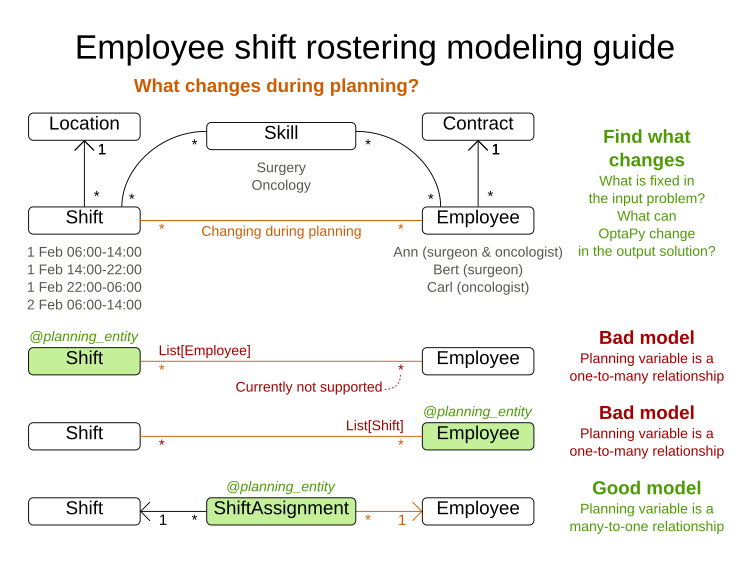
-
Annotate a many-to-one relationship with a
@planning_entityannotation. Usually the many side of the relationship is the planning entity class that contains the planning variable. If the relationship is bi-directional, both sides are a planning entity class but usually the many side has the planning variable and the one side has the shadow variable. For example, in employee rostering, theShiftAssignmentclass has an@planning_entityannotation. -
Make sure that the planning entity class has at least one problem property. A planning entity class cannot consist of only planning variables or an ID and only planning variables.
-
Remove any surplus
@planning_variabledecorators so that they become problem properties. Doing this significantly decreases the search space size and significantly increases solving efficiency. For example, in employee rostering, theShiftAssignmentclass should not annotate both theShiftandEmployeerelationship with@planning_variable. -
Make sure that when all planning variables have a value of
None, the planning entity instance is describable to the business people. Planning variables have a value ofNonewhen the planning solution is uninitialized.-
A surrogate ID does not suffice as the required minimum of one problem property.
-
There is no need to add a hard constraint to assure that two planning entities are different. They are already different due to their problem properties.
-
In some cases, multiple planning entity instances have the same set of problem properties. In such cases, it can be useful to create an extra problem property to distinguish them. For example, in employee rostering, the
ShiftAssignmentclass has the problem propertyShiftas well as the problem propertyindex_in_shiftwhich is anint.
-
-
-
Choose the model in which the number of planning entities is fixed during planning. For example, in the employee rostering, it is impossible to know in advance how many shifts each employee will have before OptaPy solves the model and the results can differ for each solution found. On the other hand, the number of employees per shift is known in advance, so it is better to make the
Shiftrelationship a problem property and theEmployeerelationship a planning variable as shown in the following examples.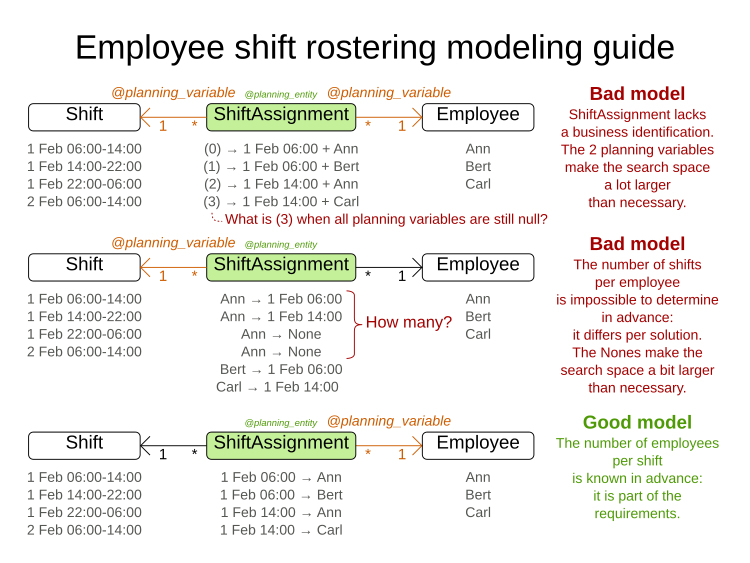
In the following diagram, each row is a different example and shows the relationship in that example’s data model. For the N Queens example, the Queen entity has a Row planning variable, which stores objects of type row. Many Queens may point to one Row.
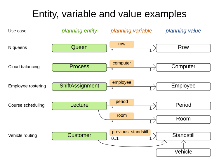
|
Vehicle routing is different because it uses a chained planning variable. |
3. Assigning time to planning entities
Dealing with time and dates in planning problems may be problematic because it is dependent on the needs of your use case.
There are several representations of timestamps, dates, durations and periods in Python. Choose the right representation type for your use case:
-
datetime.date,datetime.datetime, …: an accurate way to represent and calculate with timestamps, dates, …-
Supports timezones and DST (Daylight Saving Time).
-
-
int: Caches a timestamp as a simplified number of coarse-grained time units (such as minutes) from the start of the global planning time window or the epoch.-
For example: a
datetime.datetimeof1-JAN 08:00:00becomes anintof400minutes. Similarly1-JAN 09:00:00becomes460minutes. -
It often represents an extra field in a class, alongside the
datetime.datetimefield from which it was calculated. Thedatetime.datetimeis used for user visualization, but theintis used in the score constraints. -
It is faster in calculations, which is especially useful in the TimeGrain pattern.
-
Do not use if timezones or DST affect the score constraints.
-
There are also several designs for assigning a planning entity to a starting time (or date):
-
If the starting time is fixed beforehand, it is not a planning variable (in that solver). the arrival day of each patient is fixed beforehand.
-
This is common in multi stage planning, when the starting time has been decided already in an earlier planning stage.
-
-
If the starting time is not fixed, it is a planning variable (genuine or shadow).
-
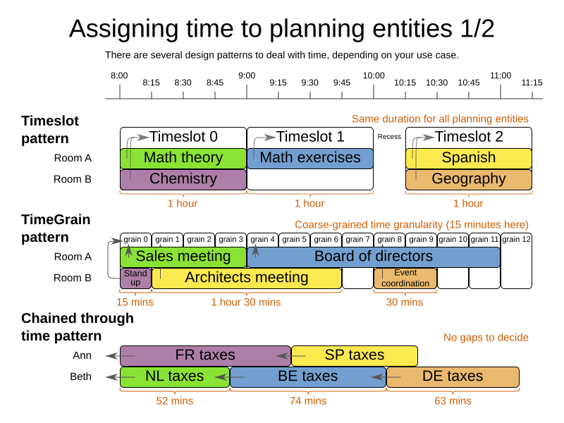
If all planning entities have the same duration, use the Timeslot pattern.
-
For example in course scheduling, all lectures take one hour. Therefore, each timeslot is one hour.
-
Even if the planning entities have different durations, but the same duration per type, it’s often appropriate.
-
For example in conference scheduling, breakout talks take one hour and lab talks take 2 hours. But there’s an enumeration of the timeslots and each timeslot only accepts one talk type.
-
-
-
If the duration differs and time is rounded to a specific time granularity (for example 5 minutes) use the TimeGrain pattern.
-
For example in meeting scheduling, all meetings start at 15 minute intervals. All meetings take 15, 30, 45, 60, 90 or 120 minutes.
-
-
If the duration differs and one task starts immediately after the previous task (assigned to the same executor) finishes, use the Chained Through Time pattern.
-
For example in time windowed vehicle routing, each vehicle departs immediately to the next customer when the delivery for the previous customer finishes.
-
Even if the next task does not always start immediately, but the gap is deterministic, it applies.
-
For example in vehicle routing, each driver departs immediately to the next customer, unless it’s the first departure after noon, in which case there’s first a 1 hour lunch.
-
-
-
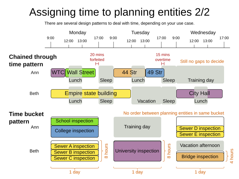
If the employees need to decide the order of theirs tasks per day, week or SCRUM sprint themselves, use the Time Bucket pattern.
-
For example in elevator maintenance scheduling, a mechanic gets up to 40 hours worth of tasks per week, but there’s no point in ordering them within 1 week because there’s likely to be disruption from entrapments or other elevator outages.
-
-
Choose the right pattern depending on the use case:
3.1. Timeslot pattern: assign to a fixed-length timeslot
If all planning entities have the same duration (or can be inflated to the same duration), the Timeslot pattern is useful. The planning entities are assigned to a timeslot rather than time. For example in course timetabling, all lectures take one hour.
The timeslots can start at any time. For example, the timeslots start at 8:00, 9:00, 10:15 (after a 15-minute break), 11:15, … They can even overlap, but that is unusual.
It is also usable if all planning entities can be inflated to the same duration. For example in exam timetabling, some exams take 90 minutes and others 120 minutes, but all timeslots are 120 minutes. When an exam of 90 minutes is assigned to a timeslot, for the remaining 30 minutes, its seats are occupied too and cannot be used by another exam.
Usually there is a second planning variable, for example the room. In course timetabling, two lectures are in conflict if they share the same room at the same timeslot. However, in exam timetabling, that is allowed, if there is enough seating capacity in the room (although mixed exam durations in the same room do inflict a soft score penalty).
3.2. TimeGrain pattern: assign to a starting TimeGrain
Assigning humans to start a meeting at four seconds after 9 o’clock is pointless because most human activities have a time granularity of five minutes or 15 minutes. Therefore it is not necessary to allow a planning entity to be assigned subsecond, second or even one minute accuracy. The five minute or 15 minutes accuracy suffices. The TimeGrain pattern models such time accuracy by partitioning time as time grains. For example in meeting scheduling, all meetings start/end in hour, half hour, or 15-minute intervals before or after each hour, therefore the optimal settings for time grains is 15 minutes.
Each planning entity is assigned to a start time grain. The end time grain is calculated by adding the duration in grains to the starting time grain. Overlap of two entities is determined by comparing their start and end time grains.
This pattern also works well with a coarser time granularity (such as days, half days, hours, …). With a finer time granularity (such as seconds, milliseconds, …) and a long time window, the value range (and therefore the search space) can become too high, which reduces efficiency and scalability. However, such a solution is not impossible, as shown in cheap time scheduling.
3.3. Chained through time pattern: assign in a chain that determines starting time
If a person or a machine continuously works on one task at a time in sequence, which means starting a task when the previous is finished (or with a deterministic delay), the Chained Through Time pattern is useful. For example, in the vehicle routing with time windows example, a vehicle drives from customer to customer (thus it handles one customer at a time).
In this pattern, the planning entities are chained. The anchor determines the starting time of its first planning entity. The second entity’s starting time is calculated based on the starting time and duration of the first entity. For example, in task assignment, Beth (the anchor) starts working at 8:00, thus her first task starts at 8:00. It lasts 52 minutes, therefore her second task starts at 8:52. The starting time of an entity is usually a shadow variable.
An anchor has only one chain. Although it is possible to split up the anchor into two separate anchors, for example split up Beth into Beth’s left hand and Beth’s right hand (because she can do two tasks at the same time), this model makes pooling resources difficult. Consequently, using this model in the exam scheduling example to allow two or more exams to use the same room at the same time is problematic.
Between planning entities, there are three ways to create gaps:
-
No gaps: This is common when the anchor is a machine. For example, a build server always starts the next job when the previous finishes, without a break.
-
Only deterministic gaps: This is common for humans. For example, any task that crosses the 10:00 barrier gets an extra 15 minutes duration so the human can take a break.
-
A deterministic gap can be subjected to complex business logic. For example in vehicle routing, a cross-continent truck driver needs to rest 15 minutes after two hours of driving (which may also occur during loading or unloading time at a customer location) and also needs to rest 10 hours after 14 hours of work.
-
-
Planning variable gaps: This is uncommon, because that extra planning variable reduces efficiency and scalability, (besides impacting the search space too).
3.3.1. Chained through time: automatic collapse
In some use case there is an overhead time for certain tasks, which can be shared by multiple tasks, of those are consecutively scheduled. Basically, the solver receives a discount if it combines those tasks.
For example when delivering pizza to two different customers, a food delivery service combines both deliveries into a single trip, if those two customers ordered from the same restaurant around the same time and live in the same part of the city.
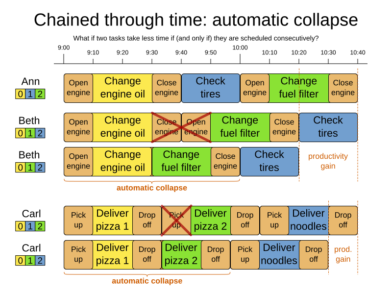
Implement the automatic collapse in the custom variable listener that calculates the start and end times of each task.
3.3.2. Chained through time: automatic delay until last
Some tasks require more than one person to execute. In such cases, both employees need to be there at the same time, before the work can start.
For example when assembling furniture, assembling a bed is a two-person job.
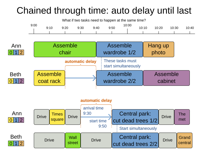
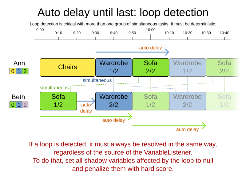
Implement the automatic delay in the custom variable listener that calculates the arrival, start and end times of each task. Separate the arrival time from the start time. Additionally, add loop detection to avoid an infinite loop:
3.4. Time bucket pattern: assign to a capacitated bucket per time period
In this pattern, the time of each employee is divided into buckets. For example 1 bucket per week. Each bucket has a capacity, depending on the FTE (Full Time Equivalent), holidays and the approved vacation of the employee. For example, a bucket usually has 40 hours for a full time employee and 20 hours for a half time employee but only 8 hours on a specific week if the employee takes vacation the rest of that week.
Each task is assigned to a bucket, which determines the employee and the coarse-grained time period for working on it. The tasks within one bucket are not ordered: it’s up to the employee to decide the order. This gives the employee more autonomy, but makes it harder to do certain optimization, such as minimize travel time between task locations.
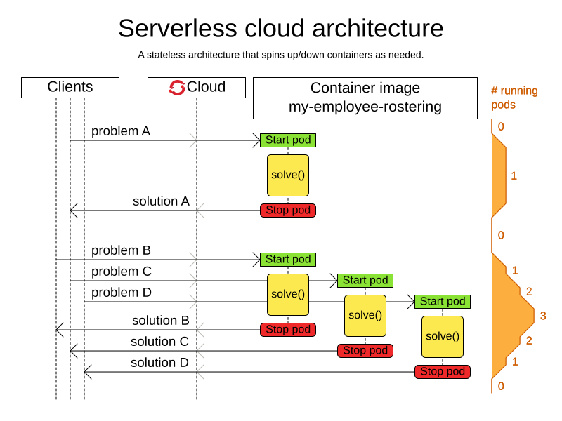
4. Cloud architecture patterns
There are two common usage patterns of OptaPy in the cloud:
-
Batch planning: Typically runs at night for hours to solve each tenant’s dataset and deliver each schedule for the upcoming day(s) or week(s). Only the final best solution is sent back to the client. This is a good fit for a serverless cloud architecture.
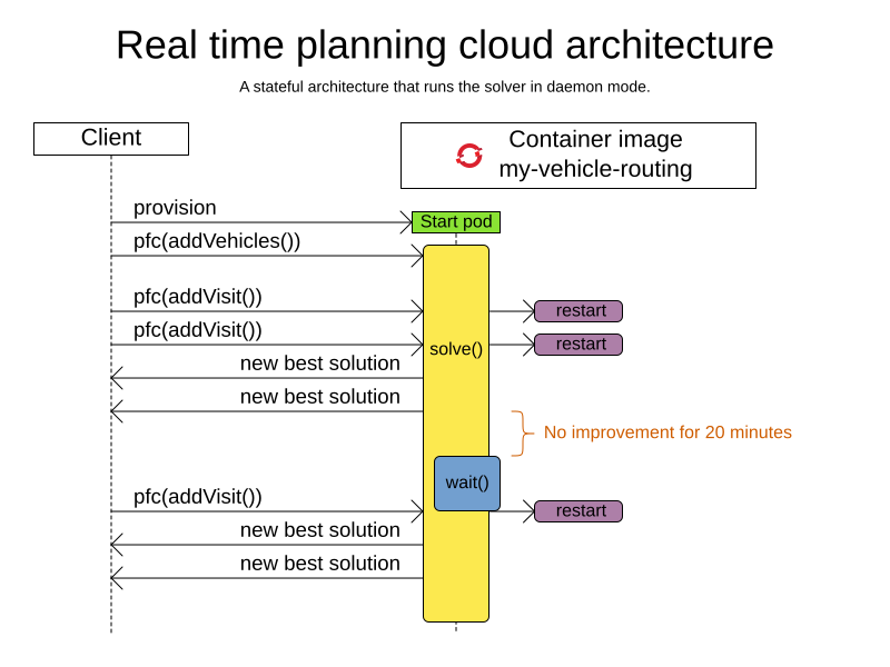
-
Real-time planning: Typically runs during the day, to handle unexpected problem changes as they occur in real-time and sends best solutions as they are discovered to the client.